

If you’ve ever worked in an office job, there’s a high chance that you have heard of Microsoft Excel at least once or twice. Whether it’s a complex database in one workbook, or a couple minor bits of information contained in one spreadsheet, Excel is a part of most office workers’ lives in one way or another. That’s why it is important to have a concrete grasp of Excel formulas that can make the sometimes-tedious work a lot easier. You may find this tool scary or feel like you don’t have the knowledge to speed up Excel’s processing needs, but we’re here to help make your existing business spreadsheets more productive and inspire some new and innovative sheets as well.
Here are 5 Excel formulas that will make any future Excel work more efficient:
1. TRIM
To start, let’s learn about some cell formatting. If your spreadsheet has unnecessary spacing from imported data, you can quickly “trim” away any excess spaces at the beginning or end of any text. It also leaves a single space between words, so no need to worry about your data being distorted.
Below is an example of what it looks like in action:
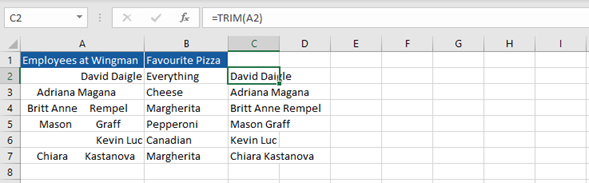
Notice how the alignment of the names is off in column A and the cells contain some unnecessary spaces. To fix this, use the TRIM function in column C. Perfectly formatted! All we need to do is copy column C and paste it into column A as text.
The TRIM function has many uses. It is especially useful when you have exported data for the purpose of an outbound direct marketing campaign via direct mail or email. The output on a direct mail piece as an example needs to be tight and precise. It can’t have a bunch of leading or following characters in the variables.
2. MIN & MAX
Next, let’s look at the MIN & MAX Excel formulas. MIN stands for minimum and gives you the smallest value from a selected range, while MAX stands for maximum, and provides the largest value. This is especially useful if you have a range of 10+ cells and it is not immediately apparent which value is which.
For example, you can use both formulas if you want to quickly determine the month of a year that had the most and least amount of revenue:
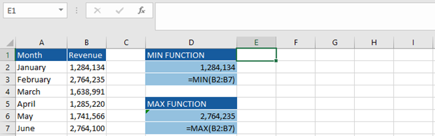
We can see the MIN formula displaying the result in cell D2, and the max formula in D6. Below these cells in D3 and D7 respectively, is the exact formula used to get these results.
3. LEFT, MID, RIGHT, LEN, and FIND
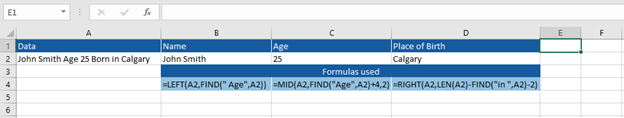
So, you’ve imported some data but only need to use a small section of information from the cell. This is where LEFT, MID, RIGHT, LEN, and FIND come in handy. These Excel formulas give you the ability to extract specific information from a cell that contains more text than you require. LEFT, MID, and RIGHT, allow you to decide where in the cell you will be getting the information. LEN gives you the length of text, and FIND quite literally finds specific text. Pretty useful, right?
You can find the formulas demonstrated below:
There’s quite a bit going on here with the combination formulas, so let’s break this down further. When you type one of the placement functions, for example LEFT, you’ll see this:
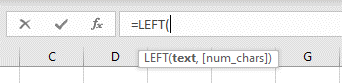
Text is asking which text you’re looking at with the formula. Here we are looking at cell A2. [Num_chars] is asking the number of characters you want to retrieve. In this case, a name can be any number of characters and so we don’t want to limit ourselves to a number. This is where the FIND function comes in.
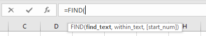
Find_text is asking what text we want to find. In this case, we want to find anything LEFT of “Age” (quotation marks are important). Within_text is once again asking which text we are looking at, and [start_num] asks for the starting position in the text, which we can leave blank here. FIND, combined with LEFT, gives us the formula and output seen in the example because we ‘found’ what was ‘left’ of age.
The same is done with the next formula using MID, but this time there are two key differences. We added +4 after find. This is because it found “Age” as a starting point, but it includes “Age” in its output. There are 4 characters (including the space) between the word “Age” and the age itself. Thus, if we add 4 it will start 4 characters away – exactly at the number. At the end for [num_chars], we put the number 2 as this is fine for our purposes (assuming the ages will two digits, so 10-99).
Finally, in this example, there is place of birth which is done using the RIGHT function. This is the same as left, except it starts right and goes left. This time for [num_chars], we started with the LEN function which returns the length of characters, in this case the length of A2. From there, we subtracted everything before “in” and then the “in” itself with the minus 2 at the end. We did it like this because we don’t know how many characters will be before “in”, and “in” is a distinct starting point for the formula.
4. IF with AND
You’ve probably heard of the IF formula. Here’s a quick recap: it gives you a value (ex. “Pass”) if a cell meets a certain condition (ex. A1>50) and an alternate value if it does not (ex. “Fail”). Now, let’s use this formula to meet some more complex conditions for your data needs. Combined with AND, the IF can narrow down your criteria further. AND can give you an extra criterion.
Take a look at the example here:
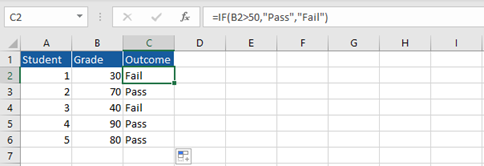
This is a simple example using the IF formula where a student passes if they get above a 50 on a test. However, let’s say we want to add a column, and only pass them if they also got above 50 on another test. Here’s how it would look:
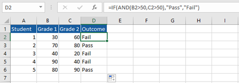
With the addition of AND, we are able to set two conditions instead of one.
5. VLOOKUP
Finally, we have the ever-mysterious VLOOKUP Excel formula. Look no further to turn this complex formula with many inputs into something you know like the back of your hand. If you have a vertically organized table somewhere in your Excel workbook, this will allow you to look up a value in the table which corresponds to another value in the same row.
Confusing? Let’s get into it with this example:
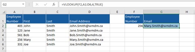
Here we had the employee number 256 and found the corresponding email from the table using VLOOKUP. To figure out how we did this, let’s examine the VLOOKUP formula.
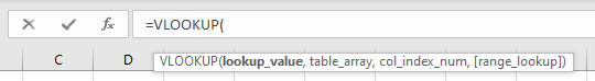
Lookup_value: What value we want to look up, could be typed in or reference a cell. Here, we referenced F2, which is the employee number we are using for our example.
Table_array: Your entire table.
Col_index_num: The number of the column you want to look in, A is 1, B is 2, and so on. Bonus: if you’re unsure of what column number you need, you can use the function COLUMN and select a cell in the column to return the number.
[Range_lookup]: Whether you want the return to be an exact match for your value or not, TRUE is an approximate match, FALSE is an exact match. In this case, it doesn’t matter.
Conclusion
This concludes our super easy guide to life-saving Excel formulas. Kidding, but they will save you time in the long run. Excel formulas are incredibly useful in streamlining work processes. Wingman Direct Marketing has extensive experience deciphering datasets and existing customer exports turning data into information and information into actionable insights. The ability to segment lists by various combination of variables and target specific customers and prospects for your communications is paramount to success in your direct mail and email campaigns.
We utilize the above formulas and many others on a daily basis. If your eyes have rolled back in your head reading the above and need someone to look at your data for you, book a Wingman today. You don’t have to fly solo.